Orthogonal projections

Spectroscopic measurements almost always contain variation that is irrelevant to the property you want to predict — baseline drift, temperature effects, scattering differences, instrument noise. Orthogonal projection methods identify this unwanted systematic variation and remove it before calibration, leaving a simpler, more interpretable dataset for the downstream model.

chemotools provides three supervised orthogonal filtering methods in chemotools.projection:

• OrthogonalSignalCorrection (OSC)

• OrthogonalPLS (OPLS)

• DirectOrthogonalization (DO)

All three are sklearn-compatible transformers: they accept (X, y) in fit and return a corrected X with the same number of features from transform. Their behaviour has been systematically compared by Svensson, Kourti & MacGregor [1].

注釈

A fourth method — ExternalParameterOrthogonalization (EPO) — handles unsupervised removal of variation linked to known external factors (e.g., temperature, humidity). It is covered on its own page.

重要

Svensson et al. [1] found that none of these methods consistently improve prediction accuracy over plain PLS on raw data. Their primary benefit is model simplicity and interpretability: the corrected data requires fewer PLS components, and the removed variation can itself carry useful diagnostic information about the measurement process.

What does "orthogonal" mean here?

After fitting a model on spectra X to predict y, the total variance in X can be decomposed into:

• Predictive variation — correlated with y, informative for the model.

• Orthogonal variation — uncorrelated with y, systematic noise or interference for the regression task.

Removing orthogonal variation before building the model reduces the number of PLS components needed and often makes the resulting loadings easier to interpret chemically.

Figure adapted from: Di Carlo, S. & Falasconi, M. "Drift Correction Methods for Gas Chemical Sensors in Artificial Olfaction Systems: Techniques and Challenges." Politecnico di Torino, Torino; SENSOR CNR-IDASC / University of Brescia, Brescia, Italy.

Choosing a method

Svensson et al. [1] identified two groups of algorithms based on how they interact with the downstream PLS model:

• Group 1 — efficient reduction (OSC variants): removing a single orthogonal component is often sufficient to substantially reduce the number of PLS components needed. One component does the work of several.

• Group 2 — one-for-one reduction (OPLS, DO): each orthogonal component removed reduces the complexity of the calibration model by exactly one PLS component.

Method	Group [1]	Iterative	Notes
OSC (wold)	1	Yes	Original formulation; can behave differently under non-linearities.
OSC (sjoblom)	1	Yes	Modified iteration; often converges faster than "wold".
OSC (fearn)	1	No	Direct, non-iterative; deterministic and fast.
OPLS	2	Yes (deflation)	Explicitly separates predictive and orthogonal variation.
DO	2	No	Projects X onto the null space of y, then extracts components via PCA.

A practical rule of thumb:

• Use OSC (fearn) as the default — it is non-iterative, deterministic, and one component is often sufficient.

• Use OPLS when you want an explicit separation of predictive and orthogonal scores for further analysis.

• Use DO as a simple, fast baseline to compare against.

警告

Extracting too many orthogonal components risks stripping predictive variation alongside the noise. Start with n_components=1 and increase only if cross-validation confirms improved model simplicity without loss of prediction accuracy.

Simulated dataset

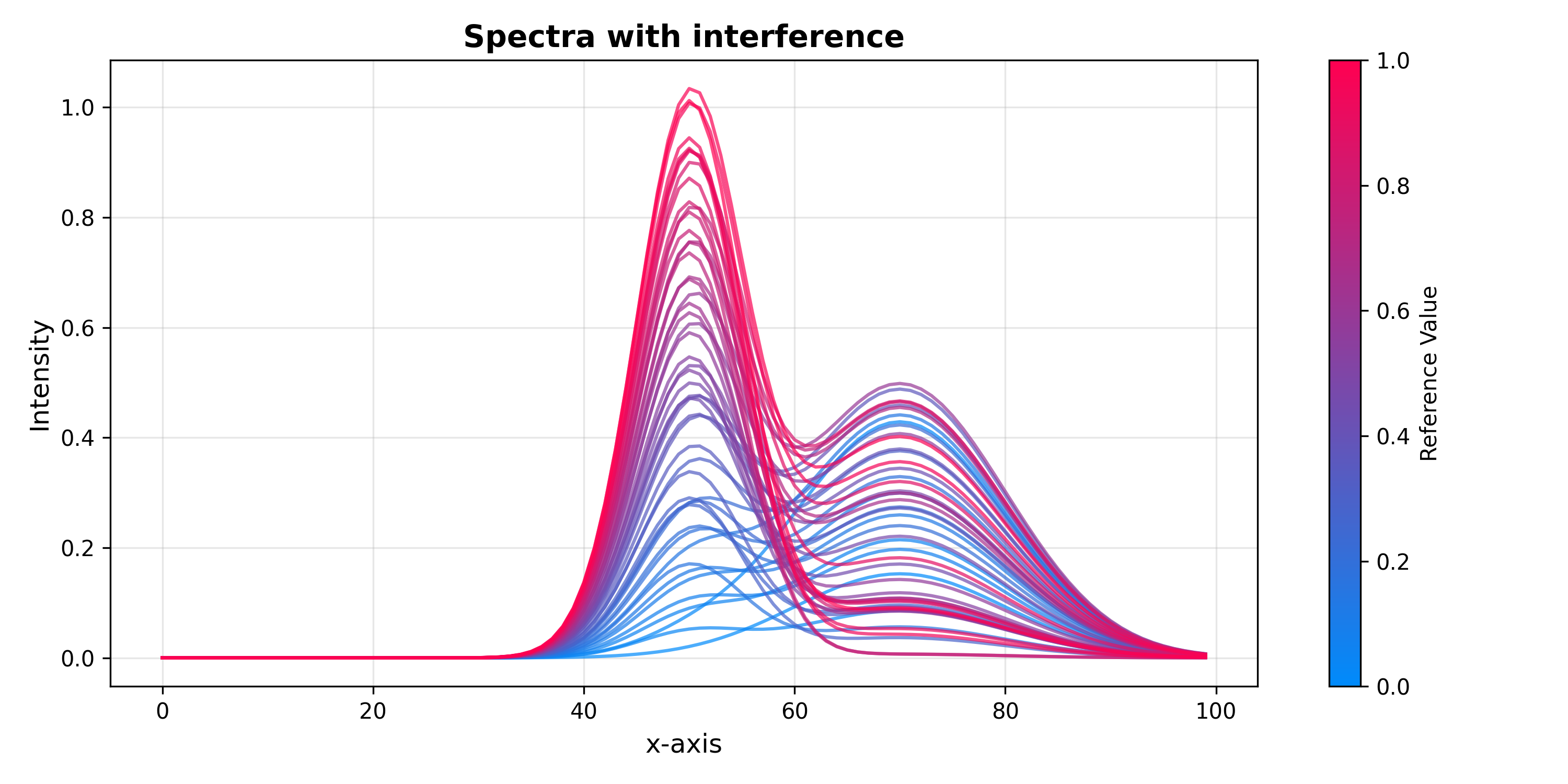
The examples below use a simple synthetic dataset where the analyte signal and the interference are known by construction — making it easy to verify visually that each method removes the right variation.

The dataset consists of 50 spectra. Each spectrum is a mixture of an analyte peak at channel 50 and an interference peak at channel 70. The analyte amplitude scales linearly with the concentration y, while the interference amplitude is drawn from a uniform distribution that is uncorrelated with y.

import numpy as np
from chemotools.plotting import SpectraPlot

rng = np.random.default_rng(42)

x_axis       = np.arange(100)
signal       = np.exp(-0.5 * ((x_axis - 50) / 5) ** 2)
interference = 0.5 * np.exp(-0.5 * ((x_axis - 70) / 10) ** 2)

y    = np.linspace(0.1, 1.0, 50)
amps = rng.random(50)
X    = np.array([y[i] * signal + amps[i] * interference for i in range(50)])

SpectraPlot(x_axis, X, color_by=y).show(
    figsize=(10, 5),
    title="Spectra with interference",
    xlabel="Channel",
    ylabel="Intensity",
)

Orthogonal Signal Correction (OSC)

Introduced by Wold et al. (1998) [2], OSC iteratively finds components in X that have maximum variance and are orthogonal to y, then removes them by deflation. It belongs to Group 1 of Svensson et al. [1]: a single component can substantially reduce the complexity of a downstream PLS model.

Three algorithmic variants are available via the method parameter:

method	Algorithm	Notes
"wold"	Iterative NIPALS-style. Alternates between score estimation and orthogonality constraint until convergence.	Original formulation [2]. Can be slow for large datasets.
"sjoblom"	Modified iteration using the pseudo-inverse of y to enforce orthogonality directly.	Often converges faster than "wold" [3].
"fearn"	Direct (non-iterative). Projects X onto the null space of y and extracts dominant components via SVD.	No convergence issues; fast and deterministic [4].

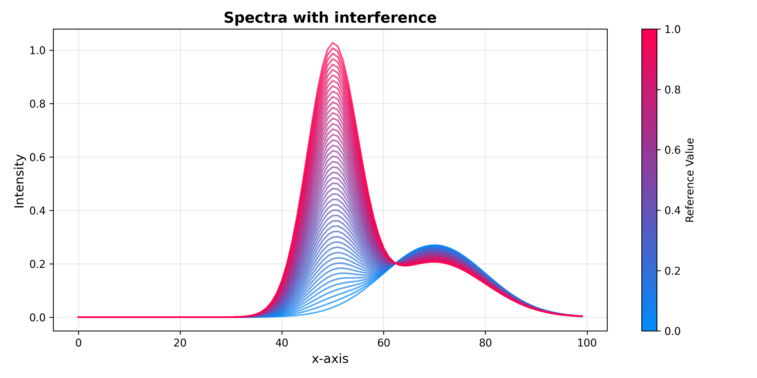
from chemotools.projection import OrthogonalSignalCorrection

osc = OrthogonalSignalCorrection(n_components=1, method="fearn")
X_osc = osc.fit_transform(X, y)

SpectraPlot(x_axis, X_osc, color_by=y).show(
    figsize=(10, 5),
    title="OSC-corrected spectra",
    xlabel="Channel",
    ylabel="Intensity",
)

Orthogonal PLS (OPLS)

Introduced by Trygg & Wold (2002) [5], OPLS extends PLS regression by explicitly separating the predictive and orthogonal components of X. It belongs to Group 2 of Svensson et al. [1]: each component removed corresponds to exactly one fewer PLS component in the downstream model.

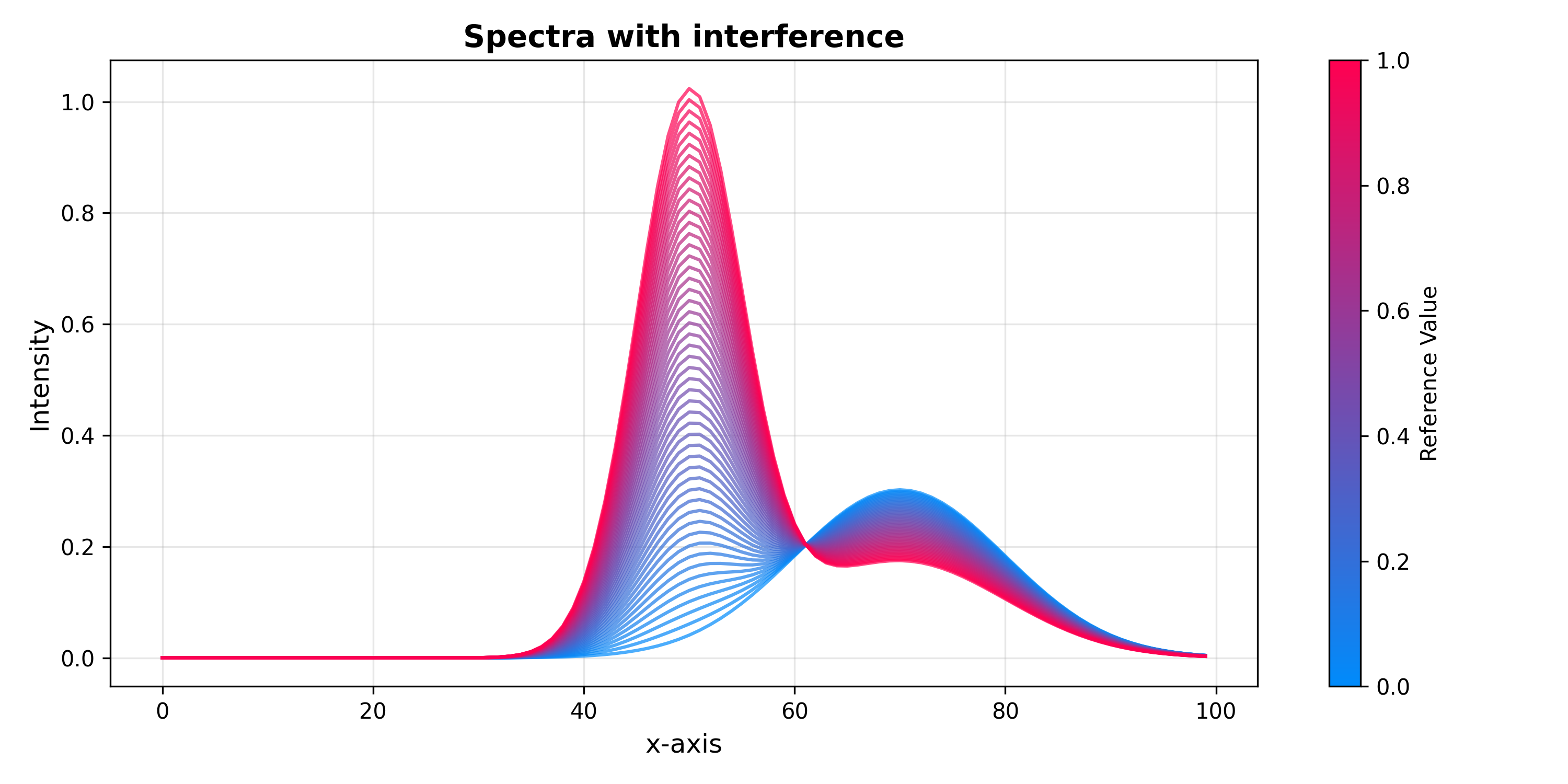
from chemotools.projection import OrthogonalPLS

opls = OrthogonalPLS(n_components=1)
X_opls = opls.fit_transform(X, y)

SpectraPlot(x_axis, X_opls, color_by=y).show(
    figsize=(10, 5),
    title="OPLS-corrected spectra",
    xlabel="Channel",
    ylabel="Intensity",
)

Direct Orthogonalization (DO)

Introduced by Andersson (1999) [6], DO is a non-iterative method. It projects X onto the null space of y to isolate the variation orthogonal to y, then extracts the dominant directions of that residual via PCA and subtracts them from the original X. Like OPLS it belongs to Group 2 of Svensson et al. [1]: one component removed equals one fewer PLS component downstream. It is computationally the lightest of the three and is useful as a fast, transparent baseline.

from chemotools.projection import DirectOrthogonalization

do = DirectOrthogonalization(n_components=1)
X_do = do.fit_transform(X, y)

SpectraPlot(x_axis, X_do, color_by=y).show(
    figsize=(10, 5),
    title="DO-corrected spectra",
    xlabel="Channel",
    ylabel="Intensity",
)

Fitting in a Pipeline

All three transformers follow the standard sklearn API and compose freely with other steps:

from sklearn.model_selection import train_test_split
from sklearn.pipeline import Pipeline
from sklearn.preprocessing import StandardScaler
from sklearn.cross_decomposition import PLSRegression
from chemotools.projection import OrthogonalSignalCorrection

X_train, X_test, y_train, y_test = train_test_split(
    X, y, test_size=0.2, random_state=42
)

pipe = Pipeline([
    ("osc",    OrthogonalSignalCorrection(n_components=1, method="fearn")),
    ("scaler", StandardScaler(with_std=False)),
    ("pls",    PLSRegression(n_components=3)),
])

pipe.fit(X_train, y_train)
y_pred = pipe.predict(X_test)

References

[1] (1,2,3,4,5,6,7)

Svensson, O., Kourti, T., & MacGregor, J. F. (2002). An investigation of orthogonal signal correction algorithms and their characteristics. Journal of Chemometrics, 16(4), 176–188. https://doi.org/10.1002/cem.700

[2] (1,2)

Wold, S., Antti, H., Lindgren, F., & Öhman, J. (1998). Orthogonal signal correction of near-infrared spectra. Chemometrics and Intelligent Laboratory Systems, 44(1–2), 175–185. https://doi.org/10.1016/S0169-7439(98)00109-9

[3]

Sjöblom, J., Svensson, O., Josefson, M., Kullberg, H., & Wold, S. (1998). An evaluation of orthogonal signal correction applied to calibration transfer of near infrared spectra. Chemometrics and Intelligent Laboratory Systems, 44(1–2), 229–244. https://doi.org/10.1016/S0169-7439(98)00112-9

[4]

Fearn, T. (2000). On orthogonal signal correction. Chemometrics and Intelligent Laboratory Systems, 50(1), 47–52. https://doi.org/10.1016/S0169-7439(99)00045-3

[5]

Trygg, J., & Wold, S. (2002). Orthogonal projections to latent structures (O-PLS). Journal of Chemometrics, 16(3), 119–128. https://doi.org/10.1002/cem.695

[6]

Andersson, C. A. (1999). Direct orthogonalization. Chemometrics and Intelligent Laboratory Systems, 47(1), 51–63. https://doi.org/10.1016/S0169-7439(98)00158-0

参考

• OrthogonalSignalCorrection

• OrthogonalPLS

• DirectOrthogonalization

• ExternalParameterOrthogonalization