モデルを検査する#
chemotools.inspector モジュールは、モデル診断のための統一インターフェースを提供します。スコア、ロードings、外れ値などのプロットを手動で作成する代わりに、Inspector が単一のメソッド呼び出しで完全な診断スイートを生成します。
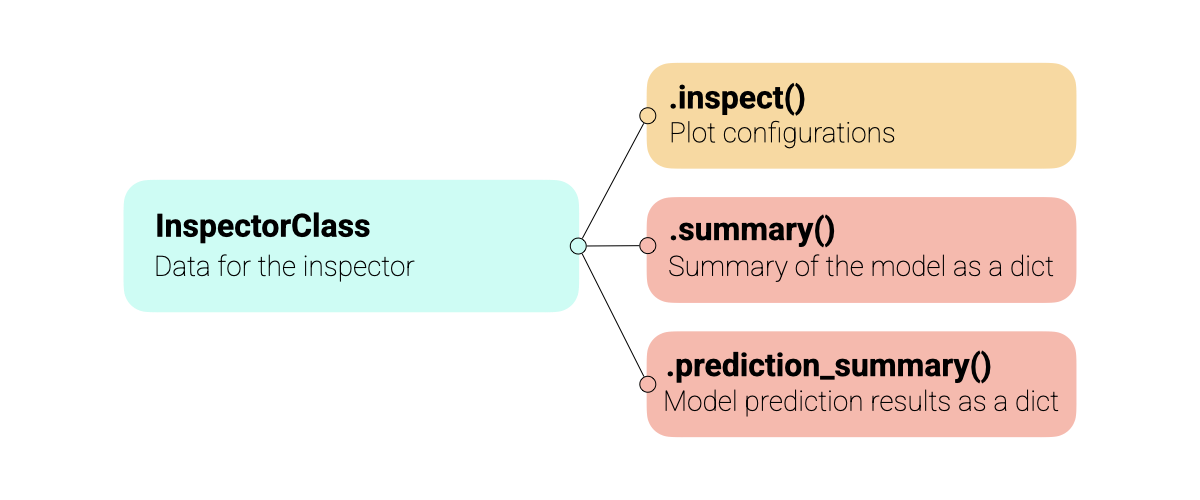
すべてのインスペクターは同じ API を共有しており、異なるモデルタイプ(PCA、PLS など)間で直感的に使用できます。インスペクターは複数のデータセット(学習、テスト、検証)をサポートし、色付け、注釈、コンポーネント選択に関する幅広いカスタマイズを提供します。以下の図はインスペクターの概要を示しています。
警告
inspector モジュールは実験的で、現在も開発が進行中です。API は将来のバージョンで変更される可能性があります。フィードバックを歓迎します。問題や提案は以下までお寄せください: paucablop/chemotools#issues
Inspector を使用する理由#
定型コードを削減し、モデルフローをより読みやすくし、モデルを十分に理解できるようにします:
ワンライナー診断:
.inspect()により、すべての標準プロット(スコア、ロードings、分散、外れ値)を生成します。統一インターフェース: PCA と PLS モデルに対して一貫した API。
マルチデータセット対応: 学習、テスト、検証データを同じプロット上で簡単に比較可能。
スペクトル比較:
.inspect_spectra()により、生データと前処理済スペクトルを比較できます。前処理の可視化:
PreprocessingInspectorを使って、パイプラインの各ステップを順に確認し、データへの影響を確認できます。データアクセス: カスタム分析のためにスコア、ロードings、係数を抽出可能。
インタラクティブ & 出版品質: カスタマイズ可能な標準 matplotlib 図を返します。
基本的な使用方法#
現時点で chemotools がサポートするインスペクターは以下の通りです:
前処理:
PreprocessingInspectorPCA:
PCAInspectorPLS 回帰:
PLSRegressionInspector
例として、いくつかのデータを読み込み、PCA と PLS 回帰モデルを学習させます。
from sklearn.cross_decomposition import PLSRegression
from sklearn.decomposition import PCA
from sklearn.pipeline import make_pipeline
from sklearn.preprocessing import StandardScaler

from chemotools.datasets import load_fermentation_train
from chemotools.derivative import SavitzkyGolay
from chemotools.feature_selection import RangeCut
from chemotools.inspector import PCAInspector, PLSRegressionInspector, PreprocessingInspector


# 1. Load Data
X, y = load_fermentation_train()
wn = X.columns

# 2. Fit the PCA Model
pca = make_pipeline(
    RangeCut(start=900, end=1400, wavenumbers=wn),
    SavitzkyGolay(window_size=21, polynomial_order=2, derivate_order=0),
    StandardScaler(with_std=False),
    PCA(n_components=3),
)
pca.fit(X)

# 3. Fit the PLS regression model
pls = make_pipeline(
    RangeCut(start=900, end=1400, wavenumbers=wn),
    SavitzkyGolay(window_size=21, polynomial_order=2, derivate_order=1),
    PLSRegression(n_components=3, scale=False),
)
pls.fit(X, y)
モデルを学習させたので、inspector を使って検査できます。モジュールの中心となるのは、すべてのインスペクターで共有されている .inspect() メソッドです。
注釈
inspect() メソッドは matplotlib.figure.Figure オブジェクトの辞書を返すため、各図を個別に保存・変更できます。
前処理ステップの検査#
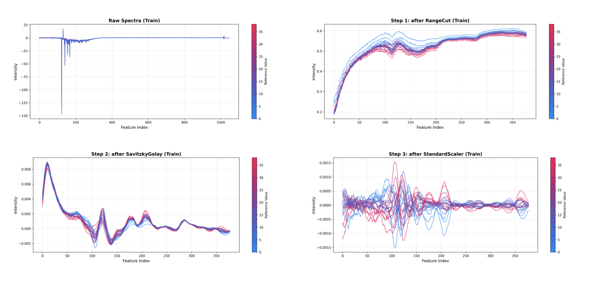
PreprocessingInspector は、パイプライン内の各前処理ステップの累積効果を可視化します。最終モデルを検査するのではなく、各変換を通じて**データがどのように変化するか**に焦点を当てます。
上で定義した同じ PCA パイプラインを使用して、各前処理ステップがデータをどのように変換するかを確認できます:
# Inspect the preprocessing steps of the PCA pipeline
inspector = PreprocessingInspector(pca, X_train=X, y_train=y, x_axis=wn)
figures = inspector.inspect()
これは前処理ステップごとに1つのプロットを生成し、生データとそれに続く各変換後の累積結果を表示します:
生スペクトル: 元の入力データ。
RangeCut 後: 関心のあるスペクトル領域を選択した後のデータ。
SavitzkyGolay 後: 平滑化されたデータ。
StandardScaler 後: 平均中心化されたデータ。
モデルステップ(例:PCA、PLS)は自動的に可視化から除外されます。
PreprocessingInspector はマルチデータセット比較もサポートしています。トレーニング、テスト、バリデーションデータを重ねて表示し、前処理がデータセット間で一貫して動作するか確認できます:
from sklearn.model_selection import train_test_split

# Split the data into training and test sets
X_train, X_test, y_train, y_test = train_test_split(
    X, y, test_size=0.2, random_state=0
)

# Initialize the inspector with both train and test data
inspector = PreprocessingInspector(
    pca,
    X_train=X_train,
    y_train=y_train,
    X_test=X_test,
    y_test=y_test,
    x_axis=wn,
)
figures = inspector.inspect(dataset=['train', 'test'])
注釈
PreprocessingInspector は、*生データ vs. 完全に前処理されたデータ*を素早く比較するための inspect_spectra() メソッドと、パイプライン情報を含む型付き dataclass を返す summary() メソッドも提供しています。
PCA モデルの検査#
次に、PCA モデルを確認します。
# Inspect the PCA model
inspector = PCAInspector(pca, X_train=X, y_train=y, x_axis=wn)
figures = inspector.inspect()
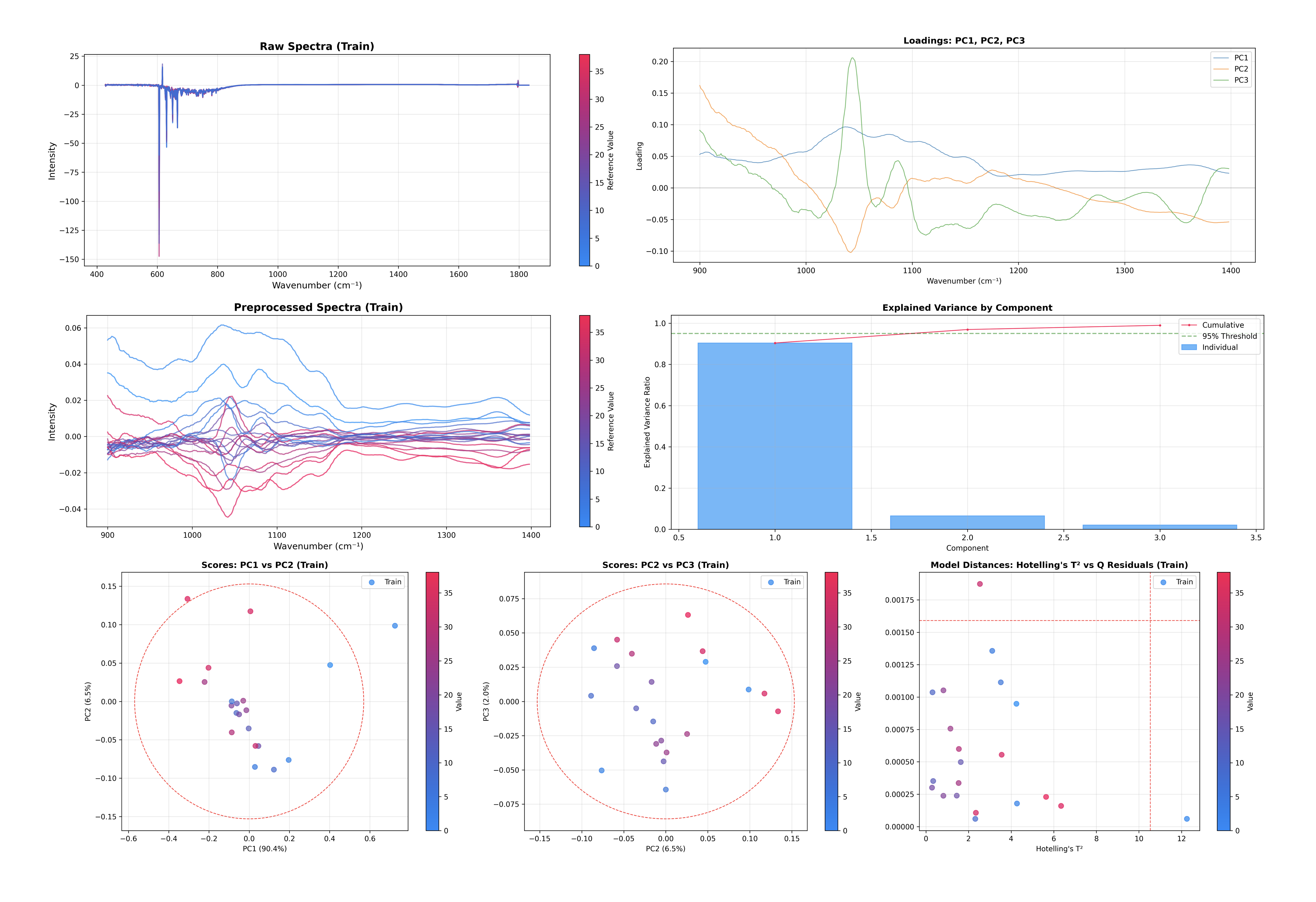
この一つのコマンドで、いくつかの重要な診断プロットが生成され、表示されます:
寄与率: コンポーネント数が十分か判断する助けとなります。
スコアプロット: サンプル空間を可視化します(PC1 vs PC2、PC2 vs PC3)。
ロードings プロット: 特徴空間(モデルが注目している特徴)を可視化します。
外れ値検出: Hotelling の T² と Q 残差のプロット。
PLS 回帰モデルの検査#
PLS 回帰インスペクターは PCAInspector と同じ API を共有しており、両者を簡単に切り替えることができます。
# Inspect the PLS Regression model
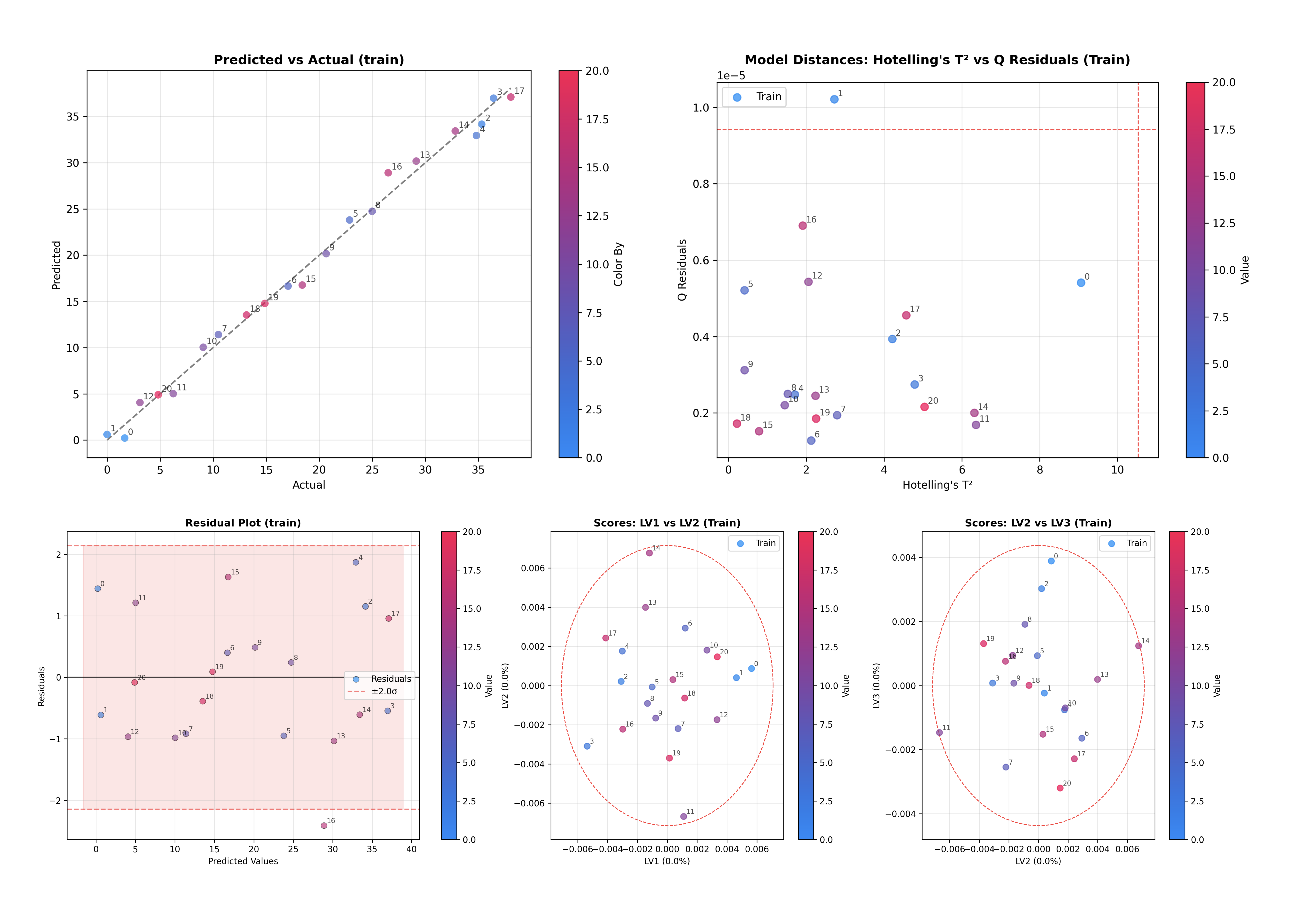
inspector = PLSRegressionInspector(pls, X_train=X, y_train=y, x_axis=wn)
figures = inspector.inspect()
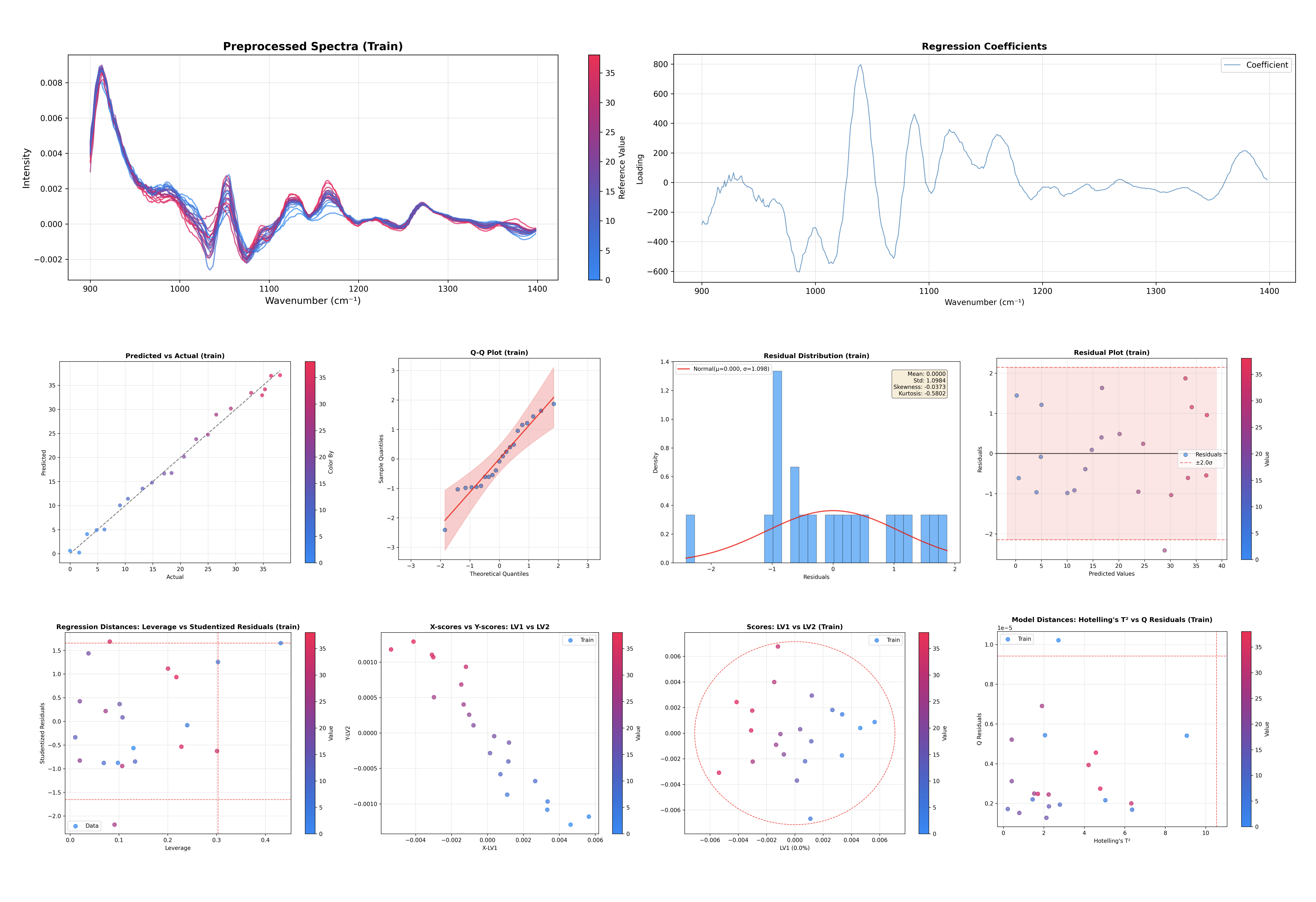
このコマンドは PLS 回帰に特化した診断プロットを生成します:
寄与率: X 空間および Y 空間に対する寄与率。
スコアプロット: サンプル空間を可視化します(LV1 vs LV2)。
X スコア vs Y スコア: 潜在変数間の相関を示します。
ロードings プロット: X ロードings、X 重み、X 回転を表示します。
回帰係数: 予測における特徴量の重要度を示します。
外れ値検出: Hotelling の T² と Q 残差のプロット。
レバレッジ vs 学生化残差: 影響力の大きいサンプルの検出。
Q 残差 vs Y 残差: モデル適合性の複合診断。
予測値 vs 実測値: 回帰性能の評価。
Y 残差プロット: 予測誤差のパターンを確認。
Q-Q プロット: 残差の正規性を確認。
残差分布: 予測誤差のヒストグラム。
スペクトルの検査#
モデルに前処理ステップ(例: sklearn Pipeline)が含まれている場合、.inspect_spectra() メソッドを使用して生スペクトルと前処理後スペクトルを比較できます:
# Compare raw vs preprocessed spectra
spectra_figures = inspector.inspect_spectra()
これにより 2 つのプロットが生成されます:
生スペクトル: 変換前の元データ。
前処理後スペクトル: すべての前処理ステップ後(モデル適用前)のデータ。
これは、前処理ステップ(ベースライン補正、微分、正規化など)が期待通りに機能しているかを確認するため、分光分析ワークフローで特に有用です。
注釈
inspect_spectra() メソッドは、前処理ステップを含む Pipeline モデルでのみ利用可能です。また、前処理が存在する場合は .inspect() によって自動的に呼び出されます。
検査のカスタマイズ#
inspect() メソッドは高いカスタマイズ性を備えており、プロットするコンポーネント、サンプルの色付け、含めるデータセットなどを指定できます。
コンポーネントの選択#
スコアプロットおよびロードings プロットで可視化するコンポーネントを指定できます。
# Plot LV2 vs LV3 for scores, and the first 2 components for loadings
inspector.inspect(
    components_scores=(1, 2),
    loadings_components=[0, 1]
)
components_scores パラメータは以下を受け付けます:
int: 最初の N 個のコンポーネントをサンプルインデックスに対してプロット
tuple (i, j): コンポーネント i とコンポーネント j のプロット
list: 複数指定、例:
[(0, 1), (1, 2)]
色付けと注釈#
デフォルトでは、プロットはターゲット変数 y に基づいて色付けされます(提供されている場合)。color_by および annotate_by パラメータを使用して、この動作をカスタマイズできます。
# Color by y and annotate by sample index
inspector.inspect(color_by='y', annotate_by='sample_index')
両パラメータは以下を受け付けます:
'y': ターゲット変数による色付けまたは注釈。'sample_index': サンプルインデックスによる色付けまたは注釈。array-like: サンプル数と同じ長さのカスタム値。
dict: データセット名を配列にマッピングしてマルチデータセットプロットを作成、例:
{'train': array1, 'test': array2}。
カラーモード#
color_mode パラメータは色の適用方法を制御します:
# Use categorical coloring (discrete colors for each unique value)
inspector.inspect(color_by='y', color_mode='categorical')

# Use continuous coloring (gradient based on values) - default
inspector.inspect(color_by='y', color_mode='continuous')
データセットの比較#
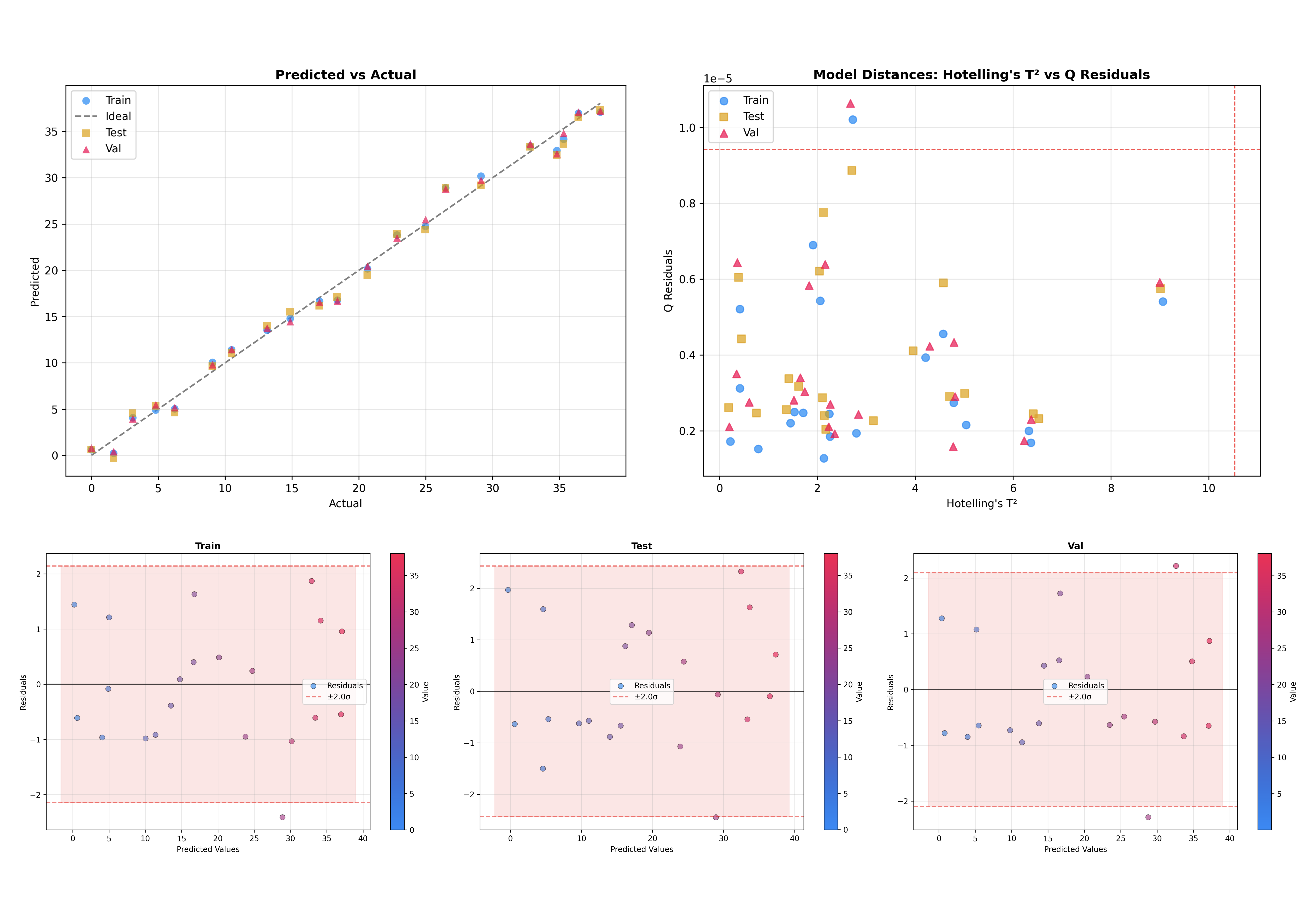
別の有用な機能として、複数のデータセットを重ねて表示できる点があります。これはモデルが未知データにどの程度一般化するか確認する上で重要です。
# Initialize inspector with train, test, and validation data
inspector = PLSRegressionInspector(
    pls,
    X_train=X_train,
    y_train=y_train,
    X_test=X_test,
    y_test=y_test,
    X_val=X_val,
    y_val=y_val,
    x_axis=wn,
)

# Inspect all datasets together
figures = inspector.inspect(dataset=['train', 'test', 'val'])
これにより、学習・テスト・検証サンプルが同一プロット上に可視化され、ドメインシフトや過学習を容易に見つけられます。
マルチ出力 PLS#
マルチ出力 PLS モデル(複数の目的変数)では、target_index パラメータを使用して検査するターゲットを選択します:
# Inspect the second target variable (index 1)
inspector.inspect(target_index=1)
プロット設定#
図のサイズを細かく制御するには、plot_config パラメータを使用するか、サイズ引数を直接渡します:
from chemotools.inspector import InspectorPlotConfig

# Using plot_config
config = InspectorPlotConfig(
    scores_figsize=(10, 8),
    loadings_figsize=(12, 4),
    variance_figsize=(8, 6),
)
inspector.inspect(plot_config=config)

# Or pass sizes directly as kwargs
inspector.inspect(scores_figsize=(10, 8))
図の操作#
inspect() メソッドは matplotlib.figure.Figure オブジェクトの辞書を返します。これにより、個々のプロットへアクセスし、さらにカスタマイズしたり、ファイルとして保存できます。
個別プロットへのアクセス#
返された辞書内の各図は記述的なキーを持ちます:
# Get all figures
figures = inspector.inspect()

# See available figure keys
print(figures.keys())
# dict_keys(['variance_x', 'variance_y', 'loadings_x', 'loadings_weights',
#            'loadings_rotations', 'regression_coefficients', 'scores_1',
#            'scores_2', 'x_vs_y_scores_1', 'distances_hotelling_q', ...])

# Access a specific figure
scores_fig = figures['scores_1']
loadings_fig = figures['loadings_x']
利用可能な図のキーはインスペクターの種類に依存します:
PCAInspector:
variance: 寄与率プロットloadings: ローディングプロットscores_1,scores_2, ...: スコアプロットdistances: Hotelling の T² 対 Q 残差
PLSRegressionInspector:
variance_x,variance_y: 寄与率プロットloadings_x,loadings_weights,loadings_rotations: ローディングプロットregression_coefficients: 回帰係数プロットscores_1,scores_2, ...: X スコアプロットx_vs_y_scores_1,x_vs_y_scores_2, ...: X 対 Y スコアプロットdistances_hotelling_q: Hotelling の T² 対 Q 残差distances_leverage_studentized: てこ比 対 学生化残差distances_q_y_residuals: Q 残差 対 Y 残差predicted_vs_actual: 予測値 対 実測値プロットresiduals: Y 残差プロットqq_plot: Q-Q プロットresidual_distribution: 残差ヒストグラムraw_spectra,preprocessed_spectra: スペクトルプロット(前処理がある場合)
図の保存#
個別の図、またはすべての図を一括で保存できます:
# Save a single figure
figures['scores_1'].savefig('scores_plot.png', dpi=300, bbox_inches='tight')

# Save as PDF for publications
figures['loadings_x'].savefig('loadings.pdf', bbox_inches='tight')

# Save all figures to a directory
import os

output_dir = 'model_diagnostics'
os.makedirs(output_dir, exist_ok=True)

for name, fig in figures.items():
    fig.savefig(f'{output_dir}/{name}.png', dpi=300, bbox_inches='tight')
図のカスタマイズ#
図は標準の matplotlib オブジェクトのため、作成後に自由に変更できます:
# Get a figure and customize it
fig = figures['scores_1']
ax = fig.axes[0]

# Modify title, labels, etc.
ax.set_title('My Custom Title', fontsize=14, fontweight='bold')
ax.set_xlabel('Latent Variable 1')
ax.set_ylabel('Latent Variable 2')

# Add annotations, lines, etc.
ax.axhline(y=0, color='gray', linestyle='--', alpha=0.5)
ax.axvline(x=0, color='gray', linestyle='--', alpha=0.5)

# Update the figure
fig.tight_layout()
モデルデータへのアクセス#
プロット以外にも、インスペクターは基礎データを抽出してカスタム分析に利用するためのメソッドを提供します。
PCA インスペクター#
inspector = PCAInspector(pca, X_train=X, y_train=y, x_axis=wn)

# Get scores for a dataset
scores = inspector.get_scores('train')  # Shape: (n_samples, n_components)

# Get loadings (optionally select components)
loadings = inspector.get_loadings()           # All components
loadings = inspector.get_loadings([0, 1])     # First two components

# Get explained variance ratio
variance = inspector.get_explained_variance_ratio()
PLS 回帰インスペクター#
inspector = PLSRegressionInspector(pls, X_train=X, y_train=y, x_axis=wn)

# X-space scores and loadings
x_scores = inspector.get_x_scores('train')
x_loadings = inspector.get_x_loadings()
x_weights = inspector.get_x_weights()
x_rotations = inspector.get_x_rotations()

# Y-space scores
y_scores = inspector.get_y_scores('train')

# Regression coefficients
coefficients = inspector.get_regression_coefficients()

# Explained variance in X and Y space
x_variance = inspector.get_explained_x_variance_ratio()
y_variance = inspector.get_explained_y_variance_ratio()
モデル概要#
インスペクターは .summary() メソッドを通じてモデルの要約統計量を提供します。これは dataclass オブジェクトを返し、.to_dict() メソッドにより辞書へ容易に変換できます。
モデルの要約#
# Get model summary
summary = inspector.summary()

# Access as object attributes
print(summary.model_type)        # 'PLSRegression'
print(summary.n_components)      # 3
print(summary.n_features)        # 1047

# Convert to dictionary
summary.to_dict()
.to_dict() メソッドは以下を返します:
{
    'model_type': 'PLSRegression',
    'has_preprocessing': True,
    'n_features': 1047,
    'n_components': 3,
    'n_samples': {'train': 21, 'test': 21, 'val': 21},
    'preprocessing_steps': [
        {'step': 1, 'name': 'rangecut', 'type': 'RangeCut'},
        {'step': 2, 'name': 'savitzkygolay', 'type': 'SavitzkyGolay'}
    ],
    'hotelling_t2_limit': 12.34,
    'q_residuals_limit': 0.56,
    'train': {'rmse': 1.07, 'r2': 0.99, 'bias': 0.01},
    'test': {'rmse': 1.21, 'r2': 0.99, 'bias': -0.02},
    ...
}
回帰指標#
PLS 回帰モデルでは、サマリーオブジェクトから回帰指標へ直接アクセスできます:
summary = inspector.summary()

# Access metrics for specific datasets
print(summary.train.rmse)    # 1.07
print(summary.train.r2)      # 0.99
print(summary.test.bias)     # -0.02
.metrics プロパティは pandas.DataFrame に最適化された構造を提供します:
import pandas as pd

# Get metrics in DataFrame-friendly format
pd.DataFrame(inspector.summary().metrics).T
| train | test | val | |
|---|---|---|---|
| rmse | 1.930431e+00 | 2.717529 | 13.107082 |
| r2 | 9.746810e-01 | 0.949825 | -0.167189 |
| bias | -8.035900e-16 | 1.882106 | -12.964854 |