Dynamic transformers#

In conventional chemometrics practice, preprocessing is treated as a static operation: a correction is determined from a calibration set and then applied uniformly to every new spectrum. The preprocessing step holds everything it needs — a stored mean spectrum, a fitted baseline, a set of PLS loadings — and the data alone is sufficient at prediction time.

This works well for a large class of problems, but it breaks down when the correction you need to apply depends on information that is only available at inference time. In practice this information falls into two categories:

Measurement metadata — instrument-level quantities recorded alongside the spectrum but not part of it: the x-axis calibration, laser power, integration time, detector temperature.
Process data — sample- or batch-level context that changes between runs or samples: a fresh background measurement, a dilution factor, a reference standard collected just before the sample or other process parameters such as temperature or humidity.

Some concrete examples from spectroscopy:

The x-axis grid of the instrument drifted between calibration and deployment. Each new spectrum arrives on a slightly different wavenumber array.
You want to normalize by laser power or integration time, values that are logged per measurement but are not part of the spectrum itself.
A background spectrum is measured fresh before each sample batch and must be subtracted at inference, not at fit time.

chemotools addresses this with a set of dynamic transformers: estimators that accept additional per-call parameters alongside X at transform time, delivered through scikit-learn’s metadata routing framework.

Dynamic transformers in `chemotools`#
Transformer	Metadata	Choose it when
`XAxisInterpolator`	`x_axis`	Spectra must be resampled from changing input grids onto one fixed grid.
`MetadataFunctionTransformer`	User-defined names	A custom correction needs one or more values that change between calls.

The distinction is useful: XAxisInterpolator is a specialized, fully validated interpolation estimator, while MetadataFunctionTransformer adapts a regular Python function to scikit-learn’s estimator and metadata-routing interfaces. Use the specialized transformer for x-axis alignment. Use the function wrapper for operations such as reference subtraction, intensity scaling, offsets, or domain-specific corrections.

XAxisInterpolator: align spectra to a common grid#

In Raman spectroscopy, each instrument has a slightly different pixel-to-wavenumber calibration. Spectra from different instruments share the same chemistry but arrive on different x-axis grids — so they cannot be stacked into a matrix until they are resampled onto a common one.

Five simulated spectra, each with a Gaussian peak at 1100 cm⁻¹ but on a slightly different grid, illustrate the problem.

Setting up the data

import numpy as np
import sklearn
import matplotlib.pyplot as plt
from chemotools.adaptation import XAxisInterpolator

sklearn.set_config(enable_metadata_routing=True)  # explained in "How metadata routing works" below

N       = 1000                   # pixels per spectrum
sigma   = 20                     # peak width (pixels)
offsets = [-10, -5, 0, 5, 10]   # pixel-grid offset per instrument

raw_spectra, raw_x_axes = [], []

for offset in offsets:
    peak = N // 2 + offset
    y = np.exp(-0.5 * ((np.arange(N) - peak) / sigma) ** 2)
    x = np.arange(N) + (1100 - peak)      # x[peak] == 1100 wn
    raw_spectra.append(y)
    raw_x_axes.append(x)

raw_spectra = np.array(raw_spectra)   # shape (5, 1000)
raw_x_axes  = np.array(raw_x_axes)    # shape (5, 1000)

Step 1 — what the instrument gives you

Each spectrum is delivered as an array of intensity values indexed by pixel number. When you plot them on a common pixel axis, the peaks appear at different positions — each instrument’s zero point is slightly different.

zoom = 40

fig, ax = plt.subplots(figsize=(6, 4))
for y in raw_spectra:
    ax.plot(y)
ax.set_xlim(N // 2 - zoom, N // 2 + zoom)
ax.set(title="Raw spectra — pixel index", xlabel="Pixel index", ylabel="Intensity")
plt.tight_layout()
plt.show()

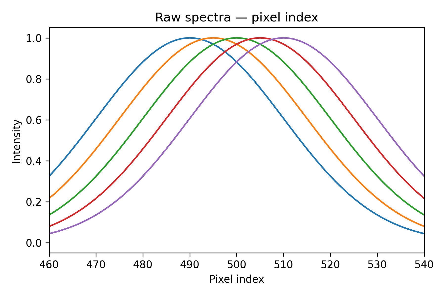
Raw spectra indexed by pixel number — peaks at different positions

Peaks land at different pixel positions — the grids are misaligned. If you stacked these rows into a matrix as-is and fed it to a PLS model, column k would represent a different wavenumber for each instrument, so every learned regression coefficient would point at the wrong feature.

Step 2 — plot against wavenumber

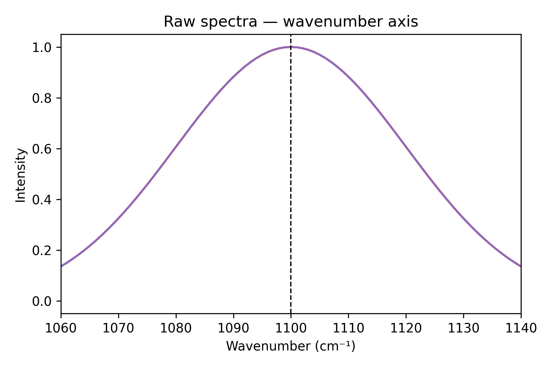
Each spectrum comes with its own wavenumber axis. Plotting against it shows the peaks coincide at 1100 cm⁻¹, but the arrays are still all different.

fig, ax = plt.subplots(figsize=(6, 4))
for y, x in zip(raw_spectra, raw_x_axes):
    ax.plot(x, y)
ax.axvline(1100, color="k", linestyle="--", linewidth=1)
ax.set_xlim(1100 - zoom, 1100 + zoom)
ax.set(title="Raw spectra — wavenumber axis", xlabel="Wavenumber (cm⁻¹)", ylabel="Intensity")
plt.tight_layout()
plt.show()

Raw spectra on their own wavenumber axes — peaks align at 1100 cm⁻¹

Step 3 — interpolate onto a common grid

XAxisInterpolator takes a common_x_axis defined once at construction time and, at every transform call, resamples each row from its own x_axis onto that shared grid. The per-spectrum axis is passed as metadata — not baked into the transformer — so it can change freely between calls.

x_common = np.linspace(650, 1550, N)

interpolator = (
    XAxisInterpolator(
        common_x_axis=x_common, method="linear", left=0, right=0
    )  # left/right fill values outside the grid
    .set_fit_request(x_axis=True)
    .set_transform_request(x_axis=True)
)

aligned_spectra = interpolator.fit_transform(raw_spectra, x_axis=raw_x_axes)

fig, ax = plt.subplots(figsize=(6, 4))
for y in aligned_spectra:
    ax.plot(y)
ax.set(
    title="Aligned spectra — common-axis index",
    xlabel="Common-axis index",
    ylabel="Intensity",
)
plt.tight_layout()
ax.set_xlim(420, 580)
plt.show()

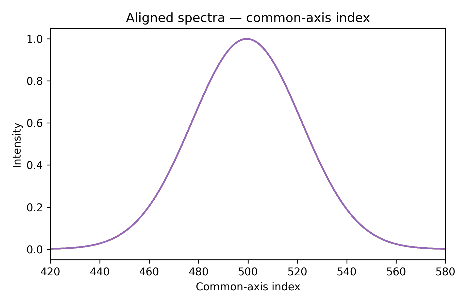
Aligned spectra on the common grid — peaks overlap perfectly

All five peaks now sit at the same column index. The matrix aligned_spectra can be fed directly into any subsequent step or model.

Route `x_axis` through a Pipeline#

The two method calls on the interpolator — set_fit_request(x_axis=True) and set_transform_request(x_axis=True) — register x_axis as a metadata argument for the fit and transform phases respectively. When you pass x_axis to a pipeline call, scikit-learn delivers it only to the step that declared it; every other step is unaffected.

set_fit_request covers fit and fit_transform; set_transform_request covers transform. Both are declared in the example because a Pipeline calling fit_transform routes metadata through both phases.

Using it inside a Pipeline#

The pipeline below continues from the same variables defined above:

from sklearn.pipeline import Pipeline
from sklearn.preprocessing import StandardScaler
from chemotools.scatter import MultiplicativeScatterCorrection

pipe = Pipeline(
    [
        (
            "interpolate",
            XAxisInterpolator(
                common_x_axis=x_common, method="linear", left=0, right=0
            )  # left/right fill values outside the grid
            .set_fit_request(x_axis=True)
            .set_transform_request(x_axis=True),
        ),
        ("msc", MultiplicativeScatterCorrection()),
        ("scaler", StandardScaler()),
    ]
)

# x_axis is routed to "interpolate" only; the other steps never see it
X_preprocessed = pipe.fit_transform(raw_spectra, x_axis=raw_x_axes)

Note

Only the step that declared set_transform_request(x_axis=True) receives x_axis. The other steps in the pipeline are unaffected.

Shared vs. per-sample grids#

Not every batch comes from multiple instruments. When all spectra in a call share the same grid, you can pass a single 1-D array instead of a matrix. x_axis accepts two shapes:

Shape (n_features,) — the same grid for every spectrum in the call. Use this when all spectra in a batch come from the same instrument (e.g., a single measurement session where the grid is fixed).
Shape (n_samples, n_features) — one grid per row. Use this when combining spectra from multiple instruments in one batch (as in the example above, where each of the five spectra has its own offset).

# Shared grid — all spectra measured on the same instrument axis
x_shared = raw_x_axes[0]                          # shape (1000,)
X_aligned_shared = interpolator.transform(raw_spectra, x_axis=x_shared)

# Per-sample grids — each spectrum has its own axis
X_aligned_per = interpolator.transform(raw_spectra, x_axis=raw_x_axes)  # shape (5, 1000)

Interpolation methods#

XAxisInterpolator supports three methods, selectable via the method parameter:

`method`	Description	When to use
`"linear"`	Piecewise linear interpolation.	Fast; best when spectra are smooth and grids are closely spaced.
`"cubic"`	Natural cubic spline (via `scipy.interpolate.CubicSpline()`).	Good all-round choice; smooth and accurate.
`"pchip"`	Piecewise cubic Hermite (via `scipy.interpolate.PchipInterpolator()`).	Preserves monotonicity; avoids overshooting near peaks.

Points outside the input grid are filled with left / right (both default to numpy.nan). You can change these to 0.0 or any other sentinel value if your downstream steps cannot handle NaN.

MetadataFunctionTransformer: build a dynamic correction#

MetadataFunctionTransformer turns a Python function into a scikit-learn transformer that can receive named metadata. It is useful when the mathematical operation is simple, but one or more operands are only known when a batch is transformed.

Consider background subtraction. A new reference spectrum is collected before each measurement batch, so it cannot be stored permanently when the model is trained. The operation itself is only X - reference. The wrapper supplies the estimator interface and routes reference to that operation at the right time.

The three pieces#

Every metadata function transformer has three parts:

The MetadataFunctionTransformer contract#
Part	Example	Meaning
Feature matrix	`X`	The first positional argument passed to the function.
Metadata names	`("reference",)`	Keyword arguments that the transformer requests and forwards.
Metadata values	`reference=background`	Values supplied separately on each transformation call.

The names must agree exactly:

def subtract_reference(X, reference):
    return X - reference

transformer = MetadataFunctionTransformer(
    func=subtract_reference,
    metadata=("reference",),
)

reference appears once in the function signature and once in the metadata tuple. Its value is supplied later:

X_corrected = transformer.fit_transform(X, reference=background)

The trailing comma in ("reference",) matters: it creates a one-item tuple. The names "X" and "y" cannot be used because they are reserved by the scikit-learn estimator API.

Start with a predefined function#

chemotools includes common, picklable functions in chemotools.adaptation.functions. Using one of these is the shortest path to a dynamic correction:

import numpy as np
from chemotools.adaptation import MetadataFunctionTransformer
from chemotools.adaptation.functions import subtract_reference

X = np.array(
    [
        [1.0, 2.0, 3.0],
        [4.0, 5.0, 6.0],
    ]
)
background = np.array([[0.2, 0.3, 0.4]])

subtract_background = MetadataFunctionTransformer(
    func=subtract_reference,
    metadata=("reference",),
)

X_corrected = subtract_background.fit_transform(
    X,
    reference=background,
)

# array([[0.8, 1.7, 2.6],
#        [3.8, 4.7, 5.6]])

The predefined functions cover four common element-wise corrections:

Predefined metadata functions#
Function	Metadata name	Operation
`subtract_reference()`	`reference`	`X - reference`
`divide_by_reference()`	`reference`	`X / reference`
`scale_by_factor()`	`factor`	`X * factor`
`add_offset()`	`offset`	`X + offset`

Understand metadata shapes#

The predefined functions use NumPy broadcasting. The metadata shape determines whether a correction is global, shared by a batch, or different for each sample.

For an input X with shape (n_samples, n_features), accepted metadata shapes are:

Metadata broadcasting patterns#
Shape	Interpretation	Typical use
Scalar	One value for every element	A global calibration factor
`(1, n_features)`	One value per feature, shared by all samples	A background spectrum for the batch
`(n_samples, 1)`	One value per sample, shared across its features	Integration time or dilution factor
`(n_samples, n_features)`	One value per element	A sample-specific reference spectrum

One-dimensional metadata is deliberately rejected by the predefined functions because its meaning is ambiguous when n_samples == n_features. Reshape it explicitly:

# One factor for each sample
factor_per_sample = factor_1d.reshape(-1, 1)

# One reference value for each feature
reference_per_feature = reference_1d.reshape(1, -1)

Custom functions decide which metadata types and shapes they support. The wrapper routes values; it does not interpret or reshape them.

Write a custom function#

A compatible function follows a small contract:

X is its first positional argument.
Routed values are named parameters that can be passed by keyword.
Every required parameter after X is listed in metadata.
It returns a finite, numeric, two-dimensional array.
It preserves the number of samples and, for this transformer, the number of features.

For example, this correction combines a per-sample integration time with an optional dark-current offset:

def correct_acquisition(X, integration_time, dark_offset=0.0):
    return (X - dark_offset) / integration_time

correction = MetadataFunctionTransformer(
    func=correct_acquisition,
    metadata=("integration_time", "dark_offset"),
)

integration_time = np.array([[1.0], [2.0]])
dark_offset = np.array([[0.05, 0.04, 0.06]])

X_corrected = correction.fit_transform(
    X,
    integration_time=integration_time,
    dark_offset=dark_offset,
)

Optional function parameters may still be listed in metadata. If no value is supplied during a direct transform call, the function’s default is used. Additional values passed to the transformer but not listed in metadata are not forwarded.

Avoid positional-only metadata parameters because metadata is always forwarded by name. In the following function, reference cannot be routed:

def incompatible(X, reference, /):
    return X - reference

Functions defined at module level are preferable to lambdas or nested functions when the fitted pipeline will be serialized. Standard pickle-based tools need to import the function by its module and name when loading the pipeline.

Validate a custom function before wrapping it#

The transformer checks the function signature during fit without executing the function. Value-dependent problems, such as an invalid metadata shape or a one-dimensional result, cannot be discovered from the signature alone.

Use check_metadata_function() with representative data to exercise the complete function contract eagerly:

from chemotools.adaptation.validation import check_metadata_function

checked_output = check_metadata_function(
    correct_acquisition,
    X,
    metadata={
        "integration_time": integration_time,
        "dark_offset": dark_offset,
    },
)

This call performs the following checks:

X is finite, numeric, and two-dimensional.
The function can be called as func(X, **metadata).
The function executes successfully on the representative values.
Its output is finite, numeric, and two-dimensional.
Its output preserves the number of samples and features.

The helper returns the validated output so the custom function is executed only once. It is intended for development, testing, and validation of a new function. It is not automatically run inside every transform call.

Warning

check_metadata_function executes user-provided code. Exceptions and side effects from the function are not suppressed.

If a custom operation intentionally changes the number of features, pass preserve_features=False to the checker. Such a function does not satisfy the same-shape contract documented by MetadataFunctionTransformer, so use that option only when the downstream interface and feature naming are handled explicitly.

Use MetadataFunctionTransformer in a Pipeline#

Enable metadata routing before passing additional values through a Pipeline:

from sklearn import set_config
from sklearn.pipeline import Pipeline
from sklearn.preprocessing import StandardScaler

set_config(enable_metadata_routing=True)

pipeline = Pipeline(
    [
        (
            "subtract_background",
            MetadataFunctionTransformer(
                func=subtract_reference,
                metadata=("reference",),
            ),
        ),
        ("scale", StandardScaler()),
    ]
)

X_ready = pipeline.fit_transform(X, reference=background)

Unlike XAxisInterpolator, the function wrapper does not require calls to set_fit_request or set_transform_request. It registers every name in metadata automatically. In this example, reference is routed to subtract_background and is not sent to StandardScaler.

After fitting, a new reference can be supplied for each prediction batch:

background_next = np.array([[0.3, 0.2, 0.4]])
X_next_ready = pipeline.transform(
    X_next,
    reference=background_next,
)

Metadata routing must be enabled for Pipeline calls, but it is not needed when calling fit_transform or transform directly on the transformer.

What happens during fit and transform#

The transformer deliberately separates structural checks from execution:

Transformer lifecycle#
Method	What it validates	What it does with metadata
`fit`	Parameters, `X`, and the callable signature	Registers names but does not execute `func`
`transform`	`X` and fitted state	Forwards listed values and executes `func` once
`fit_transform`	Performs both phases	Makes metadata available to the transformation phase

Not executing the function during fit avoids duplicate work and unexpected side effects. It also reflects the central use case: metadata values available during deployment may differ from those seen while the pipeline is fitted.

With the default validate=True, X is converted to a finite numeric two-dimensional array and its feature count is checked against the fitted input. Set validate=False only when the function must receive another data container unchanged and performs its own input validation. Output validation is always the responsibility of the function.

Common errors and how to fix them#

Choose the right dynamic transformer#

Use XAxisInterpolator when the operation is specifically interpolation from a changing source axis to a fixed target axis. It validates monotonic grids, supports multiple interpolation methods, exposes output feature names, and can process rows in parallel.

Use MetadataFunctionTransformer when the operation is naturally expressed as a function of X and one or more per-call values. Before placing a custom function in a production pipeline:

Give every routed value a clear, unique parameter name.
Test shared and per-sample metadata shapes relevant to the application.
Run check_metadata_function() on representative inputs.
Test the wrapped function through fit_transform and transform.
Use a module-level named function if the pipeline will be serialized.
Exercise the complete Pipeline with metadata routing enabled.

Together, these two estimators support pipelines that remain reusable when important correction inputs are not known until measurement or prediction time.