Inspecting your models#
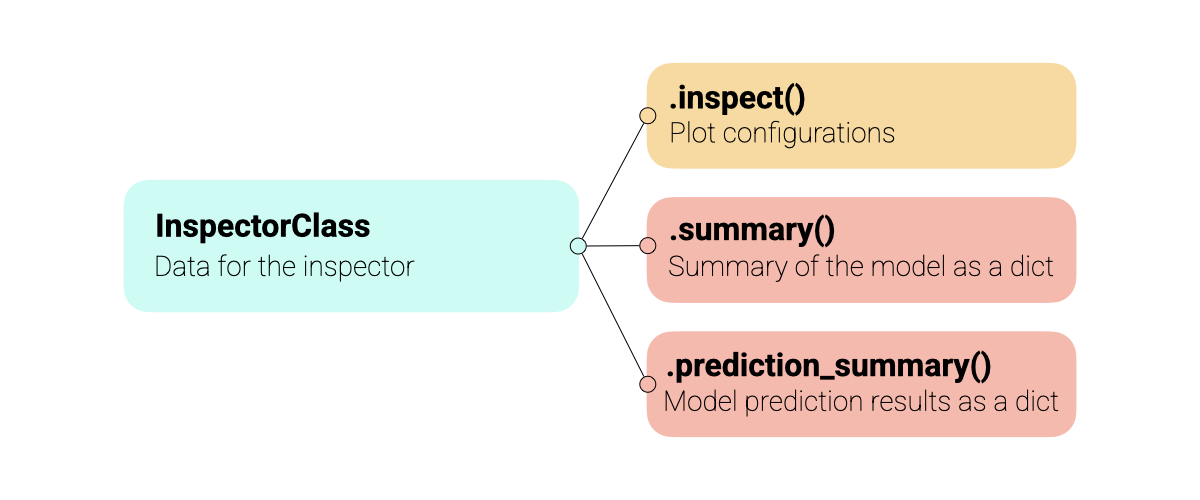
The chemotools.inspector module provides a unified interface for model diagnostics. Instead of manually creating separate plots for scores, loadings, and outliers, the Inspector generates a complete diagnostic suite with a single method call.
All inspectors share the same API, making it intuitive to use across different model types (PCA, PLS, etc.). The inspectors support multiple datasets (training, test, validation) and offer extensive customization options for coloring, annotations, and component selection. An abstract overview of the inspectors is shown in the Figure below.
Warning
The inspector module is experimental and under active development. The API may change in future versions. We welcome your feedback! Please report issues or suggestions at: paucablop/chemotools#issues
Why use the Inspector?#
Reduce boilerplate code, make your model flows more readable and ensure to fully understand your models:
One-Liner Diagnostics: Generate all standard plots (Scores, Loadings, Variance, Outliers) with
.inspect().Unified Interface: Consistent API for PCA and PLS models.
Multi-Dataset Support: Easily compare Training, Test, and Validation sets on the same plots.
Spectra Comparison: Compare raw vs preprocessed spectra with
.inspect_spectra().Preprocessing Visualization: Walk through each pipeline step and see its effect on your data with
PreprocessingInspector.Data Access: Extract scores, loadings, and coefficients for custom analysis.
Interactive & Publication Ready: Returns standard matplotlib figures that can be further customized.
Basic Usage#
Currently, chemotools supports inspectors for:
Preprocessing:
PreprocessingInspectorPCA:
PCAInspectorPLS Regression:
PLSRegressionInspector
For the example, let’s load some data and train a PCA and a PLS regression model.
from sklearn.cross_decomposition import PLSRegression
from sklearn.decomposition import PCA
from sklearn.pipeline import make_pipeline
from sklearn.preprocessing import StandardScaler

from chemotools.datasets import load_fermentation_train
from chemotools.derivative import SavitzkyGolay
from chemotools.feature_selection import RangeCut
from chemotools.inspector import PCAInspector, PLSRegressionInspector, PreprocessingInspector


# 1. Load Data
X, y = load_fermentation_train()
wn = X.columns

# 2. Fit the PCA Model
pca = make_pipeline(
    RangeCut(start=900, end=1400, wavenumbers=wn),
    SavitzkyGolay(window_size=21, polynomial_order=2, derivate_order=0),
    StandardScaler(with_std=False),
    PCA(n_components=3),
)
pca.fit(X)

# 3. Fit the PLS regression model
pls = make_pipeline(
    RangeCut(start=900, end=1400, wavenumbers=wn),
    SavitzkyGolay(window_size=21, polynomial_order=2, derivate_order=1),
    PLSRegression(n_components=3, scale=False),
)
pls.fit(X, y)
Now that we have trained the models, we can inspect them using inspector. The core of the module is the .inspect() method, shared by all inspectors.
Note
The inspect() method returns a dictionary of matplotlib.figure.Figure objects, allowing you to save or modify them individually.
Inspecting Preprocessing Steps#
The PreprocessingInspector lets you visualize the cumulative effect of each preprocessing step in a pipeline. Rather than inspecting the final model, it focuses on how your data changes through each transformation.
Using the same PCA pipeline we defined above, we can inspect how each preprocessing step transforms the data:
# Inspect the preprocessing steps of the PCA pipeline
inspector = PreprocessingInspector(pca, X_train=X, y_train=y, x_axis=wn)
figures = inspector.inspect()
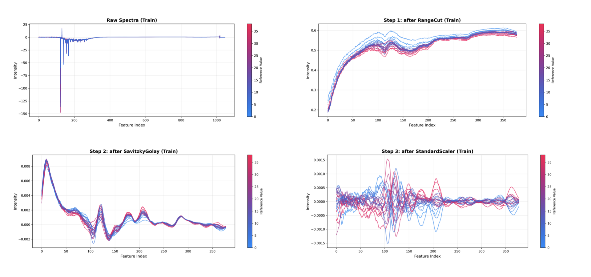
This generates one plot per preprocessing step, showing the raw data followed by the cumulative result after each transformation:
Raw Spectra: The original input data.
After RangeCut: The data after selecting the spectral region of interest.
After SavitzkyGolay: The smoothed data.
After StandardScaler: The mean-centered data.
Model steps (e.g., PCA, PLS) are automatically excluded from the visualization.
The PreprocessingInspector also supports multi-dataset comparison. You can overlay training, test, and validation data to verify that preprocessing behaves consistently across datasets:
from sklearn.model_selection import train_test_split

# Split the data into training and test sets
X_train, X_test, y_train, y_test = train_test_split(
    X, y, test_size=0.2, random_state=0
)

# Initialize the inspector with both train and test data
inspector = PreprocessingInspector(
    pca,
    X_train=X_train,
    y_train=y_train,
    X_test=X_test,
    y_test=y_test,
    x_axis=wn,
)
figures = inspector.inspect(dataset=['train', 'test'])
Note
The PreprocessingInspector also provides the inspect_spectra() method for a quick raw vs. fully preprocessed comparison, and a summary() method that returns a typed dataclass with pipeline information.
Inspecting PCA Models#
Next, we take a look at the PCA model.
# Inspect the PCA model
inspector = PCAInspector(pca, X_train=X, y_train=y, x_axis=wn)
figures = inspector.inspect()
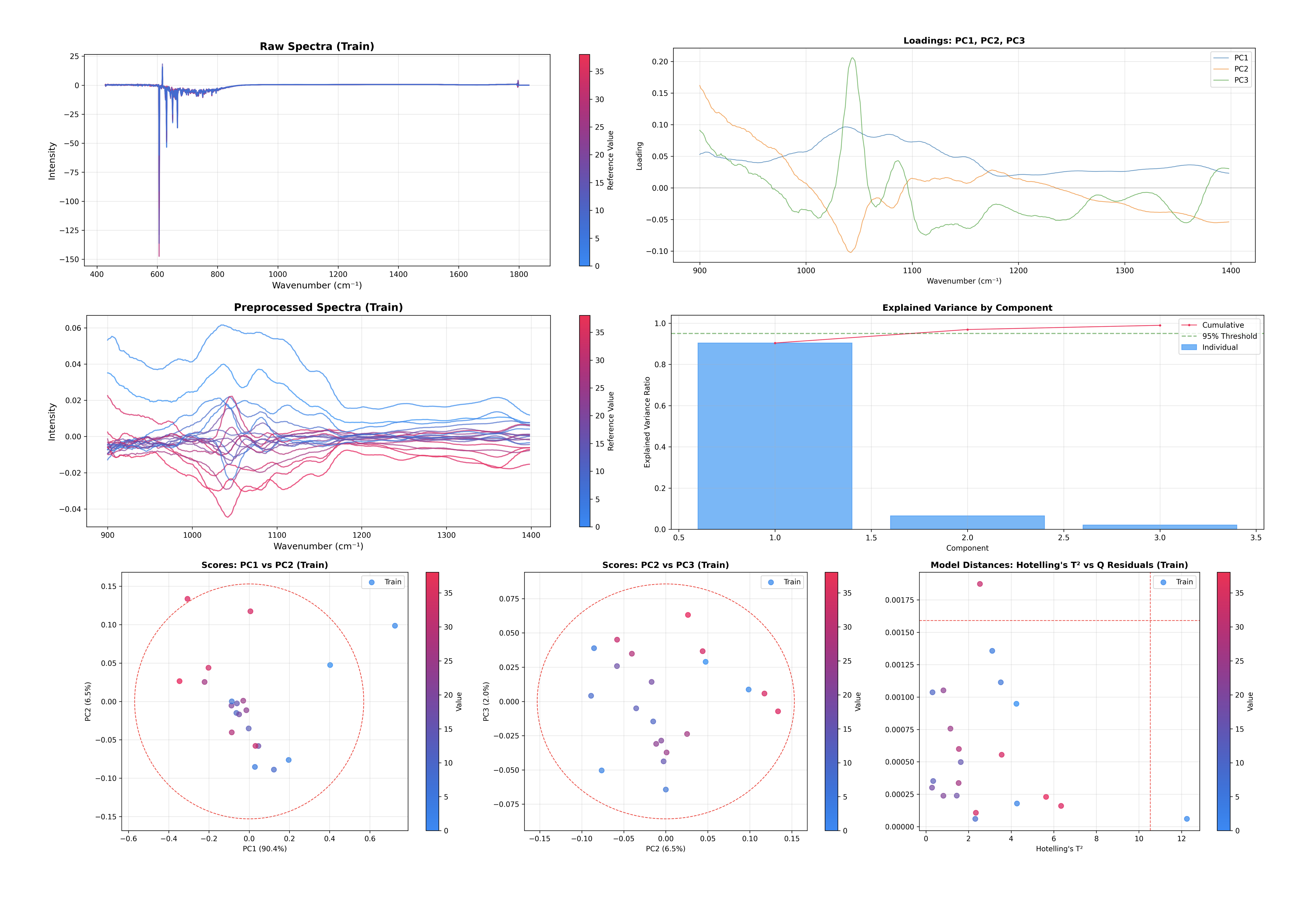
This single command generates and displays several key diagnostic plots:
Explained Variance: Helps you decide if you have enough components.
Scores Plot: Visualizes the sample space (PC1 vs PC2, PC2 vs PC3).
Loadings Plot: Visualizes the feature space (what the model is looking at).
Outlier Detection: Hotelling’s T² vs Q-Residuals plot.
Inspecting PLS Regression Models#
The PLS Regression inspector shares the same API as the PCAInspector, making it easy to switch between them.
# Inspect the PLS Regression model
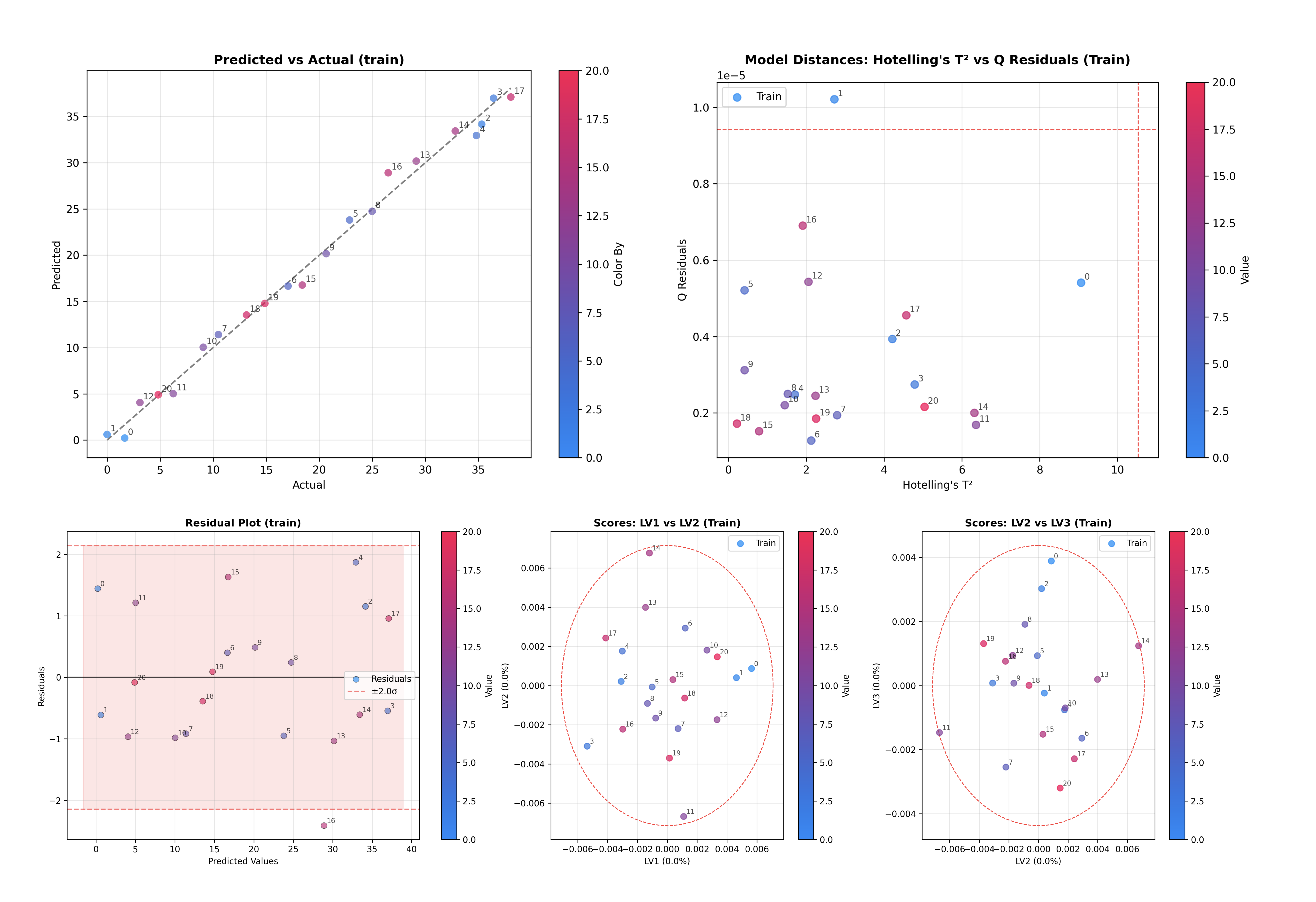
inspector = PLSRegressionInspector(pls, X_train=X, y_train=y, x_axis=wn)
figures = inspector.inspect()
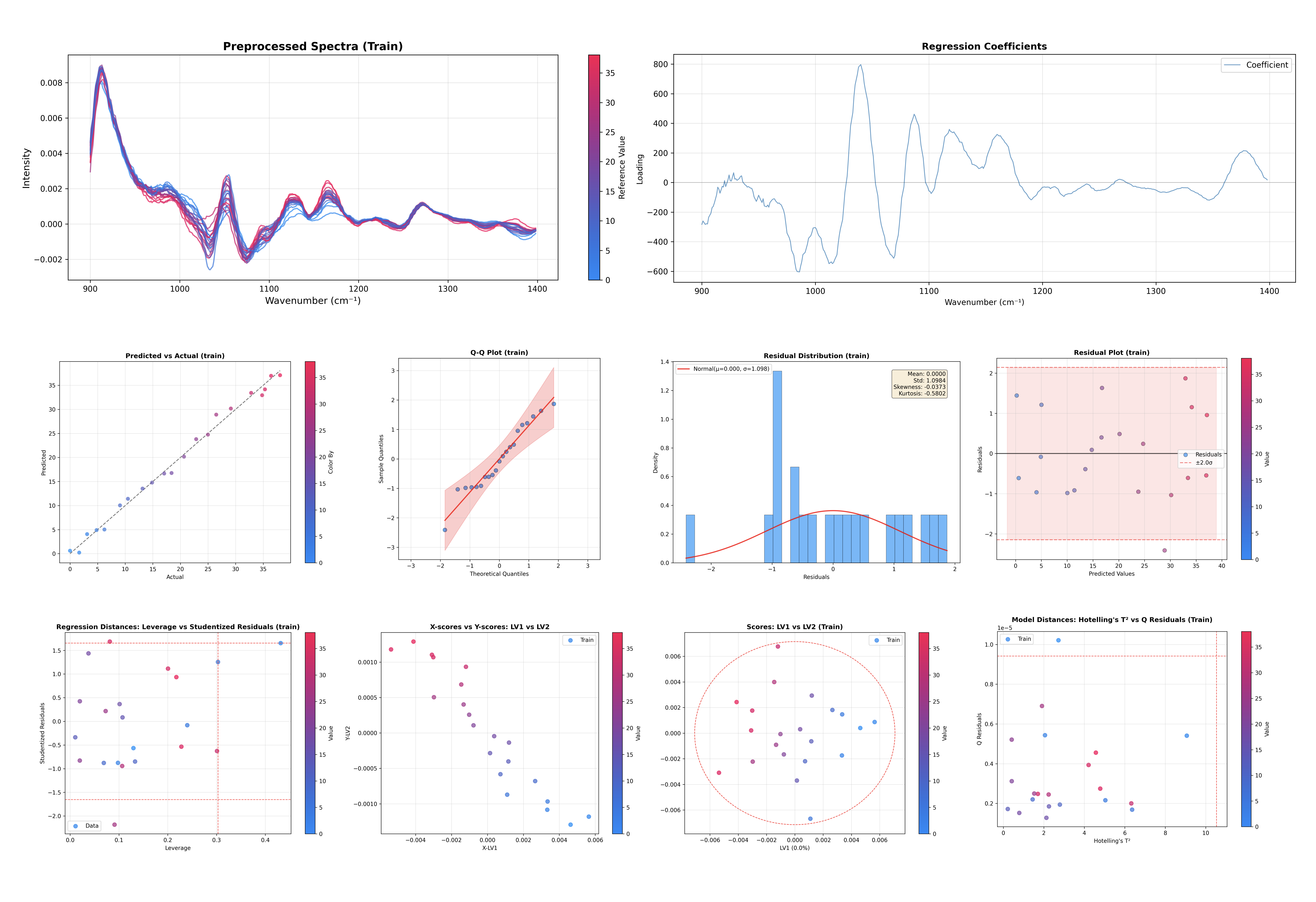
This command generates diagnostic plots tailored for PLS regression:
Explained Variance: For both X-space and Y-space.
Scores Plot: Visualizes the sample space (LV1 vs LV2).
X-Scores vs Y-Scores: Correlation between latent variables.
Loadings Plots: X-loadings, X-weights, and X-rotations.
Regression Coefficients: Feature importance for prediction.
Outlier Detection: Hotelling’s T² vs Q-Residuals plot.
Leverage vs Studentized Residuals: Influential observation detection.
Q-Residuals vs Y-Residuals: Combined model fit diagnostics.
Predicted vs Actual: Assess regression performance.
Y Residuals Plot: Identify patterns in prediction errors.
Q-Q Plot: Check normality of residuals.
Residual Distribution: Histogram of prediction errors.
Inspecting Spectra#
When your model includes preprocessing steps (e.g., a sklearn Pipeline), you can compare the raw and preprocessed spectra using the .inspect_spectra() method:
# Compare raw vs preprocessed spectra
spectra_figures = inspector.inspect_spectra()
This generates two plots:
Raw Spectra: Original input data before any transformations.
Preprocessed Spectra: Data after all preprocessing steps (before the model).
This is particularly useful in spectroscopy workflows to verify that preprocessing steps (baseline correction, derivatives, normalization) are working as expected.
Note
The inspect_spectra() method is only available when the model is a Pipeline with preprocessing steps. It is also automatically called by .inspect() when preprocessing exists.
Customizing the Inspection#
The inspect() method is highly customizable. You can control which components to plot, how to color the samples, and which datasets to include.
Selecting Components#
You can specify which components to visualize in the scores and loadings plots.
# Plot LV2 vs LV3 for scores, and the first 2 components for loadings
inspector.inspect(
    components_scores=(1, 2),
    loadings_components=[0, 1]
)
The components_scores parameter accepts:
int: Plot first N components against sample index
tuple (i, j): Plot component i vs component j
list: Multiple specifications, e.g.,
[(0, 1), (1, 2)]
Coloring and Annotations#
By default, plots are colored by the target variable y (if provided). You can customize this behavior using the color_by and annotate_by parameters.
# Color by y and annotate by sample index
inspector.inspect(color_by='y', annotate_by='sample_index')
Both parameters accept:
'y': Color/annotate by the target variable.'sample_index': Color/annotate by sample indices.array-like: Custom values of the same length as the number of samples.
dict: Map dataset names to arrays for multi-dataset plots, e.g.,
{'train': array1, 'test': array2}.
Color Mode#
The color_mode parameter controls how colors are applied:
# Use categorical coloring (discrete colors for each unique value)
inspector.inspect(color_by='y', color_mode='categorical')

# Use continuous coloring (gradient based on values) - default
inspector.inspect(color_by='y', color_mode='continuous')
Comparing Datasets#
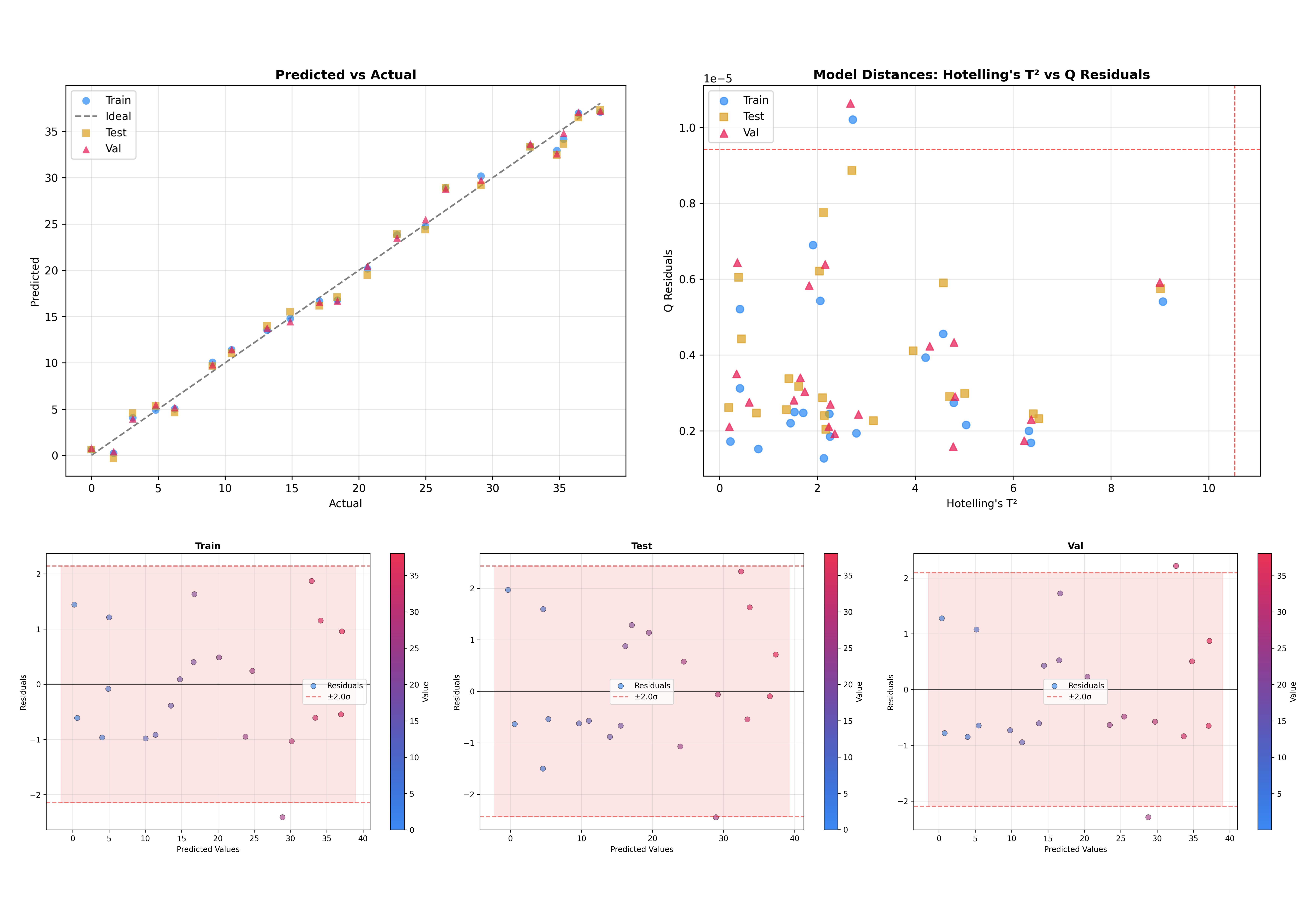
Another useful feature is the ability to overlay multiple datasets. This is critical to check how well the model generalizes to unseen data.
# Initialize inspector with train, test, and validation data
inspector = PLSRegressionInspector(
    pls,
    X_train=X_train,
    y_train=y_train,
    X_test=X_test,
    y_test=y_test,
    X_val=X_val,
    y_val=y_val,
    x_axis=wn,
)

# Inspect all datasets together
figures = inspector.inspect(dataset=['train', 'test', 'val'])
This will produce plots where training, test, and validation samples are visualized together, making it easy to spot domain shifts or overfitting.
Multi-Output PLS#
For multi-output PLS models (multiple target variables), use the target_index parameter to select which target to inspect:
# Inspect the second target variable (index 1)
inspector.inspect(target_index=1)
Plot Configuration#
For fine-grained control over figure sizes, use the plot_config parameter or pass size arguments directly:
from chemotools.inspector import InspectorPlotConfig

# Using plot_config
config = InspectorPlotConfig(
    scores_figsize=(10, 8),
    loadings_figsize=(12, 4),
    variance_figsize=(8, 6),
)
inspector.inspect(plot_config=config)

# Or pass sizes directly as kwargs
inspector.inspect(scores_figsize=(10, 8))
Working with Figures#
The inspect() method returns a dictionary of matplotlib.figure.Figure objects. This allows you to access individual plots, customize them further, or save them to files.
Accessing Individual Plots#
Each figure in the returned dictionary has a descriptive key:
# Get all figures
figures = inspector.inspect()

# See available figure keys
print(figures.keys())
# dict_keys(['variance_x', 'variance_y', 'loadings_x', 'loadings_weights',
#            'loadings_rotations', 'regression_coefficients', 'scores_1',
#            'scores_2', 'x_vs_y_scores_1', 'distances_hotelling_q', ...])

# Access a specific figure
scores_fig = figures['scores_1']
loadings_fig = figures['loadings_x']
Available figure keys depend on the inspector type:
PCAInspector:
variance: Explained variance plotloadings: Loadings plotscores_1,scores_2, …: Scores plotsdistances: Hotelling’s T² vs Q-Residuals
PLSRegressionInspector:
variance_x,variance_y: Explained variance plotsloadings_x,loadings_weights,loadings_rotations: Loadings plotsregression_coefficients: Coefficient plotscores_1,scores_2, …: X-scores plotsx_vs_y_scores_1,x_vs_y_scores_2, …: X vs Y scores plotsdistances_hotelling_q: Hotelling’s T² vs Q-Residualsdistances_leverage_studentized: Leverage vs Studentized Residualsdistances_q_y_residuals: Q-Residuals vs Y-Residualspredicted_vs_actual: Predicted vs Actual plotresiduals: Y-Residuals plotqq_plot: Q-Q plotresidual_distribution: Residual histogramraw_spectra,preprocessed_spectra: Spectra plots (if preprocessing exists)
Saving Figures#
You can save individual figures or all figures at once:
# Save a single figure
figures['scores_1'].savefig('scores_plot.png', dpi=300, bbox_inches='tight')

# Save as PDF for publications
figures['loadings_x'].savefig('loadings.pdf', bbox_inches='tight')

# Save all figures to a directory
import os

output_dir = 'model_diagnostics'
os.makedirs(output_dir, exist_ok=True)

for name, fig in figures.items():
    fig.savefig(f'{output_dir}/{name}.png', dpi=300, bbox_inches='tight')
Customizing Figures#
Since the figures are standard matplotlib objects, you can modify them after creation:
# Get a figure and customize it
fig = figures['scores_1']
ax = fig.axes[0]

# Modify title, labels, etc.
ax.set_title('My Custom Title', fontsize=14, fontweight='bold')
ax.set_xlabel('Latent Variable 1')
ax.set_ylabel('Latent Variable 2')

# Add annotations, lines, etc.
ax.axhline(y=0, color='gray', linestyle='--', alpha=0.5)
ax.axvline(x=0, color='gray', linestyle='--', alpha=0.5)

# Update the figure
fig.tight_layout()
Accessing Model Data#
Beyond plotting, the inspectors provide methods to extract underlying data for custom analysis.
PCA Inspector#
inspector = PCAInspector(pca, X_train=X, y_train=y, x_axis=wn)

# Get scores for a dataset
scores = inspector.get_scores('train')  # Shape: (n_samples, n_components)

# Get loadings (optionally select components)
loadings = inspector.get_loadings()           # All components
loadings = inspector.get_loadings([0, 1])     # First two components

# Get explained variance ratio
variance = inspector.get_explained_variance_ratio()
PLS Regression Inspector#
inspector = PLSRegressionInspector(pls, X_train=X, y_train=y, x_axis=wn)

# X-space scores and loadings
x_scores = inspector.get_x_scores('train')
x_loadings = inspector.get_x_loadings()
x_weights = inspector.get_x_weights()
x_rotations = inspector.get_x_rotations()

# Y-space scores
y_scores = inspector.get_y_scores('train')

# Regression coefficients
coefficients = inspector.get_regression_coefficients()

# Explained variance in X and Y space
x_variance = inspector.get_explained_x_variance_ratio()
y_variance = inspector.get_explained_y_variance_ratio()
Model Summaries#
The inspectors provide summary statistics of the models via the .summary() method. This returns a dataclass object with a .to_dict() method for easy conversion to dictionaries.
Model Summary#
# Get model summary
summary = inspector.summary()

# Access as object attributes
print(summary.model_type)        # 'PLSRegression'
print(summary.n_components)      # 3
print(summary.n_features)        # 1047

# Convert to dictionary
summary.to_dict()
The .to_dict() method returns:
{
    'model_type': 'PLSRegression',
    'has_preprocessing': True,
    'n_features': 1047,
    'n_components': 3,
    'n_samples': {'train': 21, 'test': 21, 'val': 21},
    'preprocessing_steps': [
        {'step': 1, 'name': 'rangecut', 'type': 'RangeCut'},
        {'step': 2, 'name': 'savitzkygolay', 'type': 'SavitzkyGolay'}
    ],
    'hotelling_t2_limit': 12.34,
    'q_residuals_limit': 0.56,
    'train': {'rmse': 1.07, 'r2': 0.99, 'bias': 0.01},
    'test': {'rmse': 1.21, 'r2': 0.99, 'bias': -0.02},
    ...
}
Regression Metrics#
For PLS regression models, you can access the regression metrics directly from the summary object:
summary = inspector.summary()

# Access metrics for specific datasets
print(summary.train.rmse)    # 1.07
print(summary.train.r2)      # 0.99
print(summary.test.bias)     # -0.02
The .metrics property provides a structure optimized for pandas.DataFrame:
import pandas as pd

# Get metrics in DataFrame-friendly format
pd.DataFrame(inspector.summary().metrics).T
| train | test | val | |
|---|---|---|---|
| rmse | 1.930431e+00 | 2.717529 | 13.107082 |
| r2 | 9.746810e-01 | 0.949825 | -0.167189 |
| bias | -8.035900e-16 | 1.882106 | -12.964854 |
See Also#
Plotting Fundamentals: For lower-level control over individual plots.
Outliers: For details on the outlier detection statistics.